[2025/01/01]내일배움캠프 QA/QC 1기 - 자습

전처리 & 시각화 3주차

df[df['sex']=='Male']

#

 

df[(df['sex']=='Male') & (df['smoker']=='Yes')]

#

 

df.loc[df['size']>3,'tip':'smoker']

#

 

df[df['size'].isin([1,2])]

#

 

df[df['day'].isin(['Sun','Thur'])]

#

df['day'] == 'Sun'

#

 

condition = df['tip'] < 2

df[condition]

#

 

cond1 = df['size'] >= 3

cond2 = df['tip'] < 2

df[cond1 & cond2]

#

 

cond = (df['sex'] == 'Male') & (df['tip'] > 3)

df[cond]

#

 

cond = (df['sex'] == 'Male') \

    & (df['tip'] > 3) & (df['smoker'] == 'Yes') \

    & (df['total_bill'] >= 20) \

    & (df['size'] == 4)

df[cond]

#

df['created_at'] = '2024-01-01'

df['created_at'] = pd.to_datetime(df['created_at'])

df

#

 

df['revenue'] = df['total_bill'] + df['tip']

df

#

 

df['tip_percentage'] = df['tip'] / df['revenue'] * 100

df

#

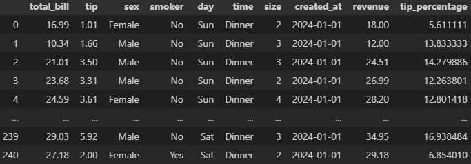
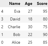
concat() : 데이터프레임을 위아래로 혹은 좌우로 연결

axis: 연결하고자 하는 축(방향)을 지정(기본값 0 - 위아래로 연결). 1로 설정하면 좌우로 연결.

ignore_index: 기본값은 False, 인덱스를 유지. True로 설정하면 새로운 인덱스를 생성. 

reset_index(drop=True)도 인덱스 새로 생성

 

concat([df1, df2, df3 ... ], axis = 0).reset_index(drop = True)

 

결측치는 NaN으로 나옴

 

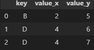
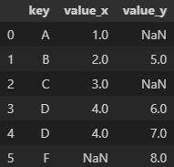
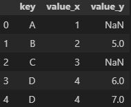
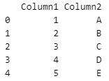
merge() : SQL의 Join과 유사한 기능. 두 개 이상의 데이터프레임에서 공통된 열이나 인덱스를 기준으로 데이터를 병합할 때 활용

데이터프레임의 순서가 중요

on : 기준이 될 컬럼 지정

left_on, right_on: 왼쪽 데이터프레임과 오른쪽 데이터프레임에서 병합할 열 이름이 다른 경우에 사용

 

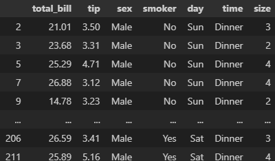
how : 병합 방법을 나타내는 매개변수. 기본값은 inner

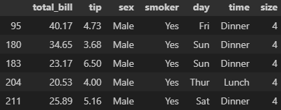
• 'inner': 공통된 키(열)를 기준으로 교집합
• 'outer': 공통된 키를 기준으로 합집합
• 'left': 왼쪽 데이터프레임의 모든 행을 포함하고 오른쪽 데이터프레임은 공통된 키에 해당하는 행만 포함
• 'right': 오른쪽 데이터프레임의 모든 행을 포함하고 왼쪽 데이터프레임은 공통된 키에 해당하는 행만 포함

 

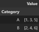
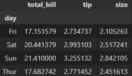
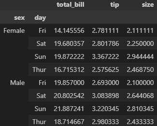
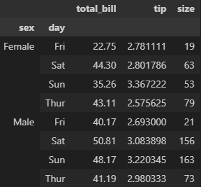
df1 = pd.DataFrame({

    'key': ['A', 'B', 'C', 'D'],

    'value': [1, 2, 3, 4]

    })

df2 = pd.DataFrame({

    'key': ['B', 'D', 'D', 'F'],

    'value': [5, 6, 7, 8]

    })

 

pd.merge(df1, df2, on = 'key')

#

 

pd.merge(df1, df2, on = 'key', how = 'outer')

#

 

pd.merge(df1, df2, on = 'key', how = 'left')

#

df = pd.DataFrame({

    'Category': ['A', 'B', 'A', 'B', 'A', 'B'],

    'Value': [1, 2, 3, 4, 5, 6]

})

df.groupby('Category').mean()

#

 

.first()

.min()

.sum() 등등

 

df.groupby('Category').agg(list)

#

 

df = pd.read_csv("temp/tips_data.csv")

df[['day','total_bill','tip','size']].groupby('day').mean()

#

 

df[['sex','day','total_bill','tip','size']].groupby(['sex','day']).mean()

#

 

df[['sex','day','total_bill','tip','size']].groupby(['sex','day']).agg({'total_bill':'max', 'tip':'mean', 'size': 'sum'})

#

 

df = pd.DataFrame({

    'Date': ['2023-01-01', '2023-01-01', '2023-01-02', '2023-01-02', '2023-01-01'],

    'Category': ['A', 'B', 'A', 'B', 'A'],

    'Value': [10, 20, 30, 40, 50]

})

pivot = df.pivot_table(index = 'Date', columns='Category', values= 'Value', aggfunc='sum')

pivot

#

df.sort_values(by='Age', ascending = False)

#

 

ascending 미작성시 기본값은 오름차순(True)

 

df.sort_values(by=['Age', 'Score'], ascending = [True,False])

#

 

df.sort_index(ascending=False)

#

pickle : python 의 변수, 함수, 객체를 파일로 저장하고 불러올 수 있는 라이브러리. binary형태로 저장되기 때문에 용량이 매우 작음

 

df = pd.DataFrame({

    'Column1': [1, 2, 3, 4, 5],

    'Column2': ['A', 'B', 'C', 'D', 'E']

})

df.to_pickle('dataframe.pkl')

loaded_df = pd.read_pickle('dataframe.pkl')

print(loaded_df)

#

import pandas as pd

import numpy as np

from datetime import datetime, timedelta

import random

# 데이터 크기 설정

num_samples = 1000

# 랜덤 시드 설정

np.random.seed(42)

# 랜덤 데이터 생성

user_ids = np.arange(1, num_samples + 1)

purchase_dates = [datetime(2023, 1, 1) + timedelta(days=np.random.randint(0, 60)) for _ in range(num_samples)]

product_ids = np.random.randint(100, 200, size=num_samples)

categories = np.random.choice(['Electronics', 'Books', 'Clothing', 'Home', 'Toys'], size=num_samples)

prices = np.round(np.random.uniform(5, 300, size=num_samples), 2)

quantities = np.random.randint(1, 6, size=num_samples)

total_spent = prices * quantities

ages = np.random.randint(18, 65, size=num_samples)

genders = np.random.choice(['M', 'F'], size=num_samples)

locations = np.random.choice(['New York', 'Los Angeles', 'Chicago', 'San Francisco', 'Houston', 'Dallas', 'Seattle', 'Austin', 'Miami', 'Boston'], size=num_samples)

membership_levels = np.random.choice(['Bronze', 'Silver', 'Gold', 'Platinum'], size=num_samples)

ad_spends = np.round(np.random.uniform(5, 50, size=num_samples), 2)

visit_durations = np.random.randint(10, 120, size=num_samples)

# 데이터프레임 생성

data = {

    'user_id': user_ids,

    'purchase_date': purchase_dates,

    'product_id': product_ids,

    'category': categories,

    'price': prices,

    'quantity': quantities,

    'total_spent': total_spent,

    'age': ages,

    'gender': genders,

    'location': locations,

    'membership_level': membership_levels,

    'ad_spend': ad_spends,

    'visit_duration': visit_durations

}

# 데이터프레임 완성

df = pd.DataFrame(data)

# 결측치 추가

nan_indices = np.random.choice(df.index, size=50, replace=False)

df.loc[nan_indices, 'price'] = np.nan

df.loc[nan_indices[:25], 'quantity'] = np.nan

# 중복 데이터 추가

duplicate_indices = np.random.choice(df.index, size=20, replace=False)

duplicates = df.loc[duplicate_indices]

df = pd.concat([df, duplicates], ignore_index=True)

# 아웃라이어 추가

outlier_indices = np.random.choice(df.index, size=10, replace=False)

df.loc[outlier_indices, 'price'] = df['price'] * 10

df.loc[outlier_indices, 'total_spent'] = df['total_spent'] * 10

# CSV 파일로 저장

df.to_csv('./user_purchase_data.csv', index=False)

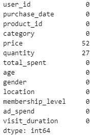
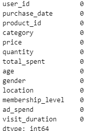
1. user_purchase_data.csv 파일에는 결측치가 포함되어 있습니다. 모든 결측치를 확인하고, 결측치가 있는 행을 제거하세요.

 

df.isnull().sum()

#

 

df = df.dropna()

df.isnull().sum()

#

 

2. purchase_date 컬럼의 데이터 타입을 문자열에서 datetime으로 변환하고, total_spent 컬럼의 데이터 타입을 정수로 변환하세요.

 

df['purchase_date'] = pd.to_datetime(df['purchase_date'])

df['total_spent'] = df['total_spent'].astype(int)

print(df.dtypes)

#

 

3. 중복된 구매 데이터를 확인하고 제거하세요. 중복의 기준은 user_id, purchase_date, product_id가 동일한 행으로 합니다.

 

4. price 컬럼에 이상치가 존재합니다. IQR (Interquartile Range) 방법을 사용하여 이상치를 찾아 제거하세요.

 

5. total_spent 컬럼을 Min-Max 정규화를 사용하여 0과 1 사이의 값으로 변환하세요.

 

3, 4, 5번은 아직 모르는 내용

4주차 강의까지 듣고 재도전

3주차 실습

데이터 홀로서기

데이터 전처리 문제

내일 다 풀기